Friday 27 June 2014

The 85+ Ways to Tie a Tie, now in Technicolor! (Knots 1 to 3)

In 1999, researchers Thomas Fink and Yong Mao at Cambridge University published a book entitled The 85 Ways to Tie a Tie. They came up with a number of criteria to limit their list of possible knots and actually published a pair of research papers on the subject in Nature and Physica A.

Not to be outdone, and disappointed that Fink and Mao ignored some pretty cool looking knots, a group of mathematicians eliminated most of the restrictions Fink and Mao had used and in 2014 published a paper proving that there were actually 177,147 ways to tie a necktie. However, even the authors had to admit that many of their knots were not very aesthetic, so it seems the criteria of Fink and Mao were not unreasonable, even if they did exclude a few good knots.

I've got a decent collection of ties and like to experiment with knots, so I've decided to work my way through all the Fink-Mao knots (plus many of the excluded knots) in this series of posts on tie knots. Click here to see a list of all the knots I've documented.

In this post I bring you knots 1 through 3, plus several variations. Almost all knots can be tied to look like the Onassis knot by either dropping the "T" from the end of the sequence of moves, or (more securely) by adding either "Li Co" or "Ri Co" to the end of the sequence. Knots can also be tied to show off what the back of the knot looks like by mirroring all the moves. Some knots look interesting in reverse and I will occasionally wear a reversed knot just to be different. I will be using the Fink-Mao notation to describe how the knots are tied. If you are unfamiliar with the notation, click on the link provided to get caught up.

Knot 1

Better known as:  Small knot, Oriental knot, Kent knot

How it's tied:  Lo Ri Co T

Additional notes: 
  • Smallest of all the tie knots. 
  • Narrow end usually extends past the wide end and will have to be hidden in some way. I usually tuck the narrow end into my shirt. 
  • Looks bad when paired with a spread collar because the collar space is way too big.
  • I find that it tends to loosen easily due to having so few moves holding it together.

What it looks like:

Kent knot (Lo Ri Co T)


Variations:
  • Onassis ending, loose (Lo Ri Co)
  • Onassis ending, secure (Lo Ri Co T Li Co)
  • Reversed knot (Ri Lo Ci T)

Kent knot, Onassis variant (Lo Ri Co)

Kent knot, Onassis variant (Lo Ri Co T Li Co)

Reverse Kent knot (Ri Lo Ci T)


Knot 2

Better known as:  Four-in-hand knot, Simple knot, Schoolboy knot

How it's tied:  Li Ro Li Co T

Additional notes: 
  • Difficult to make it look symmetrical. If you like symmetry you should probably stick to other knots.
  • A popular knot to wear loose with the collar button open.
What it looks like:

Four-in-hand knot (Li Ro Li Co T)

Variations:
  • Onassis ending, loose (Li Ro Li Co)
  • Onassis ending, secure (Li Ro Li Co T Ri Co). Most references to "Onassis knot" are referring to this particular knot.
  • Reversed knot (1/2 twist Ro Li Ro Ci T). A half twist is required before the first move in order to hide the tie's seam.

Onassis knot (Li Ro Li Co T Ri Co)

Four-in-hand knot, Onassis variant (Li Ro Li Co)


Reversed four-in-hand knot (1/2 twist Ro Li Ro Ci T)

Reversed four-in-hand knot (1/2 twist Ro Li Ro Ci T)

Knot 3

Better known as:  Kelvin knot

How it's tied:  Lo Ri Lo Ri Co T

Additional notes:  
  • Can be difficult to tie a knot that looks symmetrical
  • Has aesthetically pleasing variants known as the Cross Kelvin knot and the Diagonal knot.

What it looks like:

Kelvin knot (Lo Ri Lo Ri Co T)

Kelvin knot (Lo Ri Lo Ri Co T)


Variations:
  • Onassis ending, loose (Lo Ri Lo Ri Co)
  • Onassis ending, secure (Lo Ri Lo Ri Co T Li Co)
  • Cross Kelvin knot (Lo Ri Lo Ri Co TT)
  • Reverse Kelvin knot (Ri Lo Ri Lo Ci T)
  • Diagonal knot (reverse cross Kelvin knot) (Ri Lo Ri Lo Ci TT)

Kelvin knot with Onassis ending (Lo Ri Lo Ri Co T Li Co)
Kelvin knot with Onassis ending (Lo Ri Lo Ri Co)


Cross Kelvin knot (Lo Ri Lo Ri Co TT)


Reverse Kelvin knot (Ri Lo Ri Lo Ci T)

Reverse Kelvin knot (Ri Lo Ri Lo Ci T)


Diagonal knot (Ri Lo Ri Lo Ci TT)

Diagonal knot (Ri Lo Ri Lo Ci TT)


Tuesday 24 June 2014

Infinite Monkeys and Alphabet Permutations

Given enough time, a chimp punching keys on a typewriter at random will almost surely type out all of Shakespeare's plays.

Of course, the modern chimpanzee would choose a laptop over a typewriter for this task.

This metaphor describes what's known as the "infinite monkey theorem", which basically states that any finite string of characters must be contained within an infinite string of random characters. Here's the proof:

Let's start with looking at the probability of typing a particular finite string of letters on the first try. Let's also ignore all the other keys on a typewriter (or keyboard for those of you who've never seen a typewriter) and consider just the 26 letters of the alphabet. There is a 1 in 26 chance of any particular letter being typed. We are assuming that the letters are selected randomly and independently, so the chance of typing any two particular letters is (1/26) * (1/26) = 1 in 676. Any three particular letters: (1/26)³ = 1 in 17,576. For some number "k" particular letters: 1 in 26 to the k-th power. Now the probability of the inverse situation - not typing a particular letter (or block of letters) - is simply 100% minus the probability of successfully typing a particular letter (or block of letters). I've summarized in the tables below and included notes to help you understand the magnitudes of some of the numbers.


It's clear that randomly typing a short word on the first attempt is extremely unlikely. A complete sentence is practically impossible from our perspective. The chances of typing complete book at random are so exceedingly small that a physical analogy doesn't exist. Let's go off on a bit of tangent to look at some really big and really small numbers in the physical universe. The observable universe is a sphere with a diameter of approximately 92 billion light years, or (to employ some of Mr. Spock's absurd precision) approximately 870,387,203,477,433,600,000,000,000 metres. The Planck length represents the shortest length that, theoretically, could ever possibly be measured. It's approximately equal to 0.000 000 000 000 000 000 000 000 000 000 000 016 161 99 metre. However difficult to fathom the magnitudes of these numbers might be, just keep in mind that I can still fit them on one line in this blog post without resorting to scientific notation. The number representing the chance of successfully typing Hamlet at random on the first attempt contains 55,059 more digits than the play Hamlet does letters. Similarly, the number representing the chance of successfully typing the Bible at random on the first attempt contains 1,467,549 more digits than the Bible does letters. Here are some other really big and really small numbers to show just how small the observable universe is compared to the number of ways you can fail to type a complete work of fiction at random:


Ok, back to proving the infinite monkey theorem. We've calculated the chances of typing a string of k letters on the first attempt. What if we had more monkeys? Let's say there are M monkeys, each with a MacBook Air to type their random strings of letters. The probability of at least one of M monkeys successfully typing a particular string of k letters at random on the first attempt is:


The limit of p as M approaches infinity is 100%:


This means that, given enough monkeys typing randomly, the probability that at least one will successfully type a particular string of k letters on the first attempt approaches 100%. We can also rearrange the equation above to solve for the number of monkeys necessary to ensure a given likelihood that at least one monkey will be successful on the first attempt:


I've calculated how large M has to be to give a certain probability of success by at least one of the monkeys and summarized below.

Number of monkeys required to ensure a given probability of success on the first attempt.

The numbers of monkeys needed to achieve a reasonable probability of success are mindbogglingly large, but they are still finite and calculable.

Ok, we've seen what happens with many monkeys, but we can look at this in a different way. What if instead of many monkeys, we have a single monkey with infinite lifespan, typing randomly and continuously. This problem is a little more interesting and the exact probability is a function of the particular pattern we're looking for. First I'll demonstrate how the probability depends on the particular pattern. Suppose you're playing "Penney's Game" with a fair coin and want to know the chances of getting the sequence HHH or THH in a continuous sequence of tosses. The chance of getting either in the first 3 tosses is equal to 1/2 * 1/2 * 1/2 = 1/8. But as you keep going, the likelihood of THH increases because you have more potential starting points. Let's look at HHH. If you get one H, there's a 50% chance that the next toss is an H, and an equal chance it's a T. Now if you toss a second H, you have a 50% chance of completing the sequence, but if you toss a T, you have to wait at least one more toss to start over with another H. Put another way, if you're trying to get HHH but toss H and then T, you have to toss at least three more times to succeed in getting HHH. When you're after THH, if you toss a T and then another T, you're still potentially only two tosses away from success. In either case, your chance of success approaches 100% as your total number of tosses increases, but THH approaches 100% faster than HHH.


The same situation occurs with our random letters of the alphabet. The probability of finding a certain sequence of letters in a continuous random sequence depends on the sequence that you're looking for. However, the effect is less significant here because there are 26 possible outcomes per keystroke instead of just 2 and the finite string we're really after is thousands of characters long. Consider the pairs of letters AA and AS. They have equal chance of appearing in the first two letters (0.148%) of a random sequence. However, in a random three-letter sequence, AS has a 0.290% chance of appearance, compared to 0.284% for AA.

Despite the complication, there is still hope for our analysis of the monkey that ceaselessly types random letters. We can estimate a very conservative lower bound on the probability by dividing the sequence of n letters into n/k non-overlapping blocks. This basically assumes that the string we're searching for must start at some multiple of k-letters into the full sequence.

Conservative lower bound probability

Now it'd be nice if we had an upper bound on the probability. I can't prove that this is an upper bound, and it might not necessarily always be an upper bound, but I think that it is probably likely to be an upper bound. Instead of assuming there are n/k independent trial starting points, let's assume that every letter is an independent trial starting point. Then subtract (k -1) so that we eliminate the final few letters as possible starting points (because if you start fewer than k letters from the end, you can't possibly complete the string). To give an example, if the string is PAS, you can't possibly get PAS at the end of a random letter sequence if the third-to-last letter is not 'P'. So that gives us an estimated upper limit of n - k + 1 independent trials.

Upper bound (?) probability

The limit of both of these equations as n approaches infinity is 100%. This confirms that after typing a sufficient number of letters at random, the probability that you happened to type some finite string of letters approaches 100%.


We can also take the upper and lower bound probability and estimate the number of letters the monkey would have to type to achieve a given probability of  success.

The high estimate of n, based on the low estimate of p.

The low estimate of n, based on the high estimate of p.

Total number of letters required in the sequence to ensure a given probability of matching a string of k letters.

So is there any conceivable way we could actually type something like Hamlet at random? Let's forget about our metaphorical monkeys now and discuss this in terms of computing power. CPU speeds today are commonly on the order of 3 GHz. A computer with a 3 GHz CPU would not actually be able to generate random letters at a rate of 3 billion per second, but I'll be very conservative anyway to demonstrate how unlikely it is that the randomly duplicated work of fiction will ever exist. Let's assume that our computers will be able to generate random letters indefinitely at a rate of 3,000,000,000,000,000,000 (3 billion billion) letters per second. According to this 2008 article, there were over 1 billion PCs in use at the time and there would be an estimated 2 billion in use by 2014. So let's be really conservative and assume that we employ 4,000,000,000,000,000,000 (4 billion billion) computers with the task of generating random works of literature. I'll even use the upper bound probability estimate here. How long would it take before we had a reasonable probability that at least one computer matched a particular string of letters at least once? Well putting it all together gives us this lovely looking equation to estimate the probability of success at any time t (in seconds) after embarking on this endeavor:

Approximate probability of success after t seconds in our hypothetical scenario.

Solving for t from the approximate equation above gives us:


Which gives us an estimated lower bound time limit on matching a particular string of k letters. The number of years it would take before we could reasonably expect a duplication of Hamlet is still mindbogglingly large (it contains 187,694 digits!). The estimated age of the universe is only an 11 digit number of years (about 13.8 billion years). Even matching a complete sentence would take thousands of years.


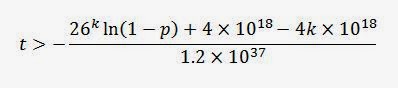
Okay, let's give it one more chance. Surely the universe could duplicate Hamlet if we could enlist alien races to help out. The number of stars in the universe is estimated to be between 10 to the 22nd and 10 to the 24th powers. Let's take 100 times the high estimate and assume 10 to the 26th power. Now let's assume that 10 intelligent races exist around each star and match the computing power from our previous hypothetical scenario, and that we all coordinate to devote our total computing power to duplicating Hamlet by random letter selection. So in a grand universal waste of time, effort, and resources, we've employed {4 followed by 45 zeroes} computers spitting out random letters at a rate of 3 billion billion letters per second each. Now p and t are:


And we still can't duplicate Hamlet within 100 billion years with only a 1 in 1,000,000 probability. In fact, we probably can't even duplicate a short paragraph.

Conservative estimate of the minimum time required to match a particular string of letters
with given probability using the universe's combined computing power.

So there you have it. By the Infinite Monkey Theorem, duplication of Shakespeare's work is possible with enough computing power. However, actual duplication is practically impossible from a physical perspective.

Epilogue

In 2003 the University of Plymouth actually spent grant money (about 2,000 British pounds, equal to about $3,270 USD or $4,580 CAD at the time) to give a computer to six macaques for a month and study their "literary output". The monkeys produced only five pages of text, apparently were fond of the letter 'S', and preferred using the computer as a lavatory to doing any actual typing. Even when they were typing, they made lousy random letter generators. Some confused creationists, such as this one, have used the results of this "study" as evidence against evolution. First, they fail to recognize that the monkeys in the "infinite monkey theorem" metaphor are meant to represent unthinking generators of random events, not actual monkeys. Actual monkeys do not act randomly. Their past experiences and their environmental conditions will influence their actions. Second, the study involved only six monkeys sharing one computer for only one month. That's hardly enough time or "monkey power" to generate a random string of letters long enough to expect anything resembling a word, let alone an entire work of fiction. Anyone who thinks this study tells us anything useful about the infinite monkey theorem is making the absurd assumption that either six monkeys is approximately equal to infinite monkeys or one month is approximately equal to infinite time.

Monday 23 June 2014

Gambling and Expected Value: Crown and Anchor

In this post on Gambling and Expected Value, we look at the game Crown and Anchor.
Click here to find similar posts on other lotteries and games of chance.


How the Game Works

The game Crown and Anchor is a dice game that historically was often played by British sailors. Instead of ordinary dice, each face has one of six symbols: crown, anchor, spade, diamond, club, and heart.


A Crown and Anchor mat with dice.

Players can bet on one or more symbols coming up and then roll three dice. If the symbol you bet on comes up, you win. The payout depends on how many of the dice are showing the symbol. 

There is also a variant of the game played with a wheel instead of dice. The wheel is divided into 216 segments, where each segment shows one the 216 possible ways to choose from the six symbols three times. The banker in this case spins the wheel and the winner is determined based on which segment is showing when the wheel stops.

Probabilities and Prizes

If the winning symbol appears on one of the three dice, the payout is 1:1 on the wager. If two of the three dice are showing the winning symbol, it's a 2:1 payout. Likewise, if all three dice are showing the symbol, it's a 3:1 payout. So there are four possible outcomes for a wager (loss, 1:1 payout, 2:1 payout, and 3:1 payout). Each die has 6 symbols, so there are 6 * 6 * 6 = 216 possible combinations of symbols when three dice are rolled. The probability of losing is 5/6 * 5/6 * 5/6 = 125/216. That leaves 91 possible ways to win (approximately a 42% chance of winning something). Only one of those combinations would be all three symbols matching the wager. Therefore, there's a 1 in 216 chance of winning the 3:1 payout. There are 15 possible ways to get exactly two matching symbols, so there is a 15 in 216 = 5 in 72 chance of winning the 2:1 payout. Finally, there are 75 ways to get exactly one matching symbol, corresponding to a 75 in 216 = 25 in 72 chance of winning the 1:1 payout.


Expected Value

The expected value of Crown and Anchor is about -$0.079 per dollar wagered, which was calculated as follows:


This means that, on average, you lose nearly 8 cents of every dollar wagered. A lot better than lotteries or Monte or 50/50 draws, allowing you to play longer with your money. It's much more comparable to casino games, though there are other options with even better expected value.

Saturday 14 June 2014

Gambling and Expected Value: Three-Card Monte

In this post on Gambling and Expected Value, we look at Three-Card Monte.
Click here to find similar posts on other lotteries and games of chance.


How the Game Works

The game Three-Card Monte is typically just a con to sucker anyone dumb enough to play out of all their money, but we're going to assume for this blog post that we're dealing with a completely fair version of the game. A dealer has three cards on a table, a "money card" and two others. The money card is typically the Queen of Hearts and the other cards are typically the Jack of Spades and Jack of Clubs. A player is asked to bet that they can find the money card after the dealer has turned the cards face down and expertly re-arranged them. The player guesses which card is the Queen and wins if he guesses correctly. The wager is lost if the player is wrong. 

Probabilities and Prizes

The player is generally led to believe that if he watches closely, he can follow the Queen at all times and know where it ends up when the dealer is done shuffling. However, during shuffling a skilled dealer stacks up two cards in one hand and can throw either the bottom card or the top card down at will. When executed correctly, the player can't tell which of the two cards was thrown. Therefore, it becomes a game of chance for the player rather than a game of skill. There is a 1 in 3 chance of revealing the money card, which pays out 1:1 on the wager.


Expected Value

The expected value of a fair version of Three-Card Monte is easy to calculate because there is only one way to play and only two possible outcomes. There's a 1 in 3 chance of winning the wager and 2 in 3 chance of losing it. Therefore, the expected value is -1/3 times the wager. In other words, for every dollar wagered, on average, you're losing a third of it.


So playing Three-Card Monte is a good way to throw money away even if the game is played fairly. However, if played fairly, Three-Card Monte is a smarter gamble than 50/50 draws or lotteries. That said, keep in mind this analysis was merely hypothetical. Three-Card Monte is a con game and a number of tricks are used to ensure that the player never wins a single bet. In other words, your true expected value in a realistic game is -1, or at least much closer to -1 than my hypothetical analysis suggests.

Sunday 1 June 2014

Gambling and Expected Value: 50/50 Draws

In this post on Gambling and Expected Value, we look at 50/50 draws.
Click here to find similar posts on other lotteries and games of chance.


How the Game Works

Players purchase tickets and their money goes into a prize pool. The prize pool is equal to 50% of the total ticket revenue. The other half of the revenue goes to whoever coordinated the draw. One ticket is drawn and the matching ticket holder wins the jackpot. 50/50 draws are often held at fundraiser events (half of the revenue goes to support some cause and half goes to the jackpot winner). 

Probabilities and Prizes

Let's say a ticket costs C dollars and N tickets are sold. The prize is equal to 0.5*C*N and each ticket has a 1/N chance of winning.

Simple enough. But what happens when there's a multi-ticket discount available? It is often the case that as an incentive to sell more tickets, a lower unit price is set if you buy a larger number of tickets. For example, $2 each or 3 for $5. Won't that mess around with the formulas above? Well, yes, a little bit.

Let's say that the single-ticket price is C1 and that there's some lower unit price available C2 = αC1, where α is some factor between 0 and 1. In the example I gave, C1 would be $2 and C2 would be $1.67, making α = 0.833. Let's also say that the number of tickets sold at the higher price is N1 and the number of tickets sold at the lower price is N2βN1
The total number of tickets sold is:
and the total ticket revenue is:
The prize pool is half of the ticket revenue:
and the probability of any ticket being drawn is:

The table below gives the prize pool for different values of α and β per 1,000 total tickets sold:

Expected Value

The expected value of the 50/50 draw ticket is the weighted average outcome, which is the probability of winning multiplied by the net gain plus the probability of losing multiplied by the cost of the ticket:
So, the prize increases with ticket sales, the probability of winning decreases with ticket sales, but the number of tickets sold doesn't influence the expected value. In the simple 50/50 draw where all tickets are bought at the same price, on average, you're losing half of the ticket price on every ticket purchased.

Now when there are two price points, the expected value depends on how many tickets were sold at each price and the relative difference in the two prices. The expected value of a ticket bought at C1 is:
Because α is between 0 and 1 and β is non-negative, we can conclude that EV1 is negative for all values of α and β. In fact, we could go step further and show that it is always between -0.5*C1 and -C1.

Moving on to the expected value of a ticket bought at C2:
EV2 is interesting because it is not necessarily always negative like EV1. If the person setting the ticket prices doesn't know any better, he or she might choose α < 0.5, in which case EV2 could potentially be positive, a dream come true for the intelligent gambler. It can be shown that EV2 is bounded between -0.5*C1 and +0.5*C1
Well a positive expected value sounds pretty good, but we need to look further. Under what conditions are we getting the maximum expected value? The partial derivatives of EV2 will tell us. 
The partial derivative with respect to β is negative for all values of α between 0 and 1. That means that EV2 always decreases as β increases. The maximum expected value must occur when β is minimized. β = 0. The partial derivative with respect to α is also negative for all permissible values of β. This means that EV2 always decreases as α increases, so the maximum expected value must occur when α is minimized. α = 0. 

So far there's been a lot of math and no pretty pictures, so here are the expected values EV1 and EV2 plotted at different values of α and β:
Expected value of a 50/50 draw ticket per $1 price C1.

As you can see from the plot, both EV1 and EV2 decrease as β increases, and both approach -0.50 as α approaches 1.0 (which makes sense because α = 1 is the simple case where there's a single ticket price). Both EV1 and EV2 are per $1 of ticket price C1. In the graph I normalized both expected values by dividing by C1 because at allows for all 9 of the plotted curves to be resolved for a larger range of β. Furthermore, EV2/C2 = 0/0 for all values of β if α = 0. That isn't very informative and can't be plotted. However, we ought to be comparing EV1/C1 to EV2/C2, as shown in the plot and tables below:


Now what does all this math mean to someone in the real world? Technically, a positive expected value is possible for a ticket purchased at C2, but only under unrealistic conditions. β must be less than 1/α - 2, but greater than zero (β < 0 makes no physical sense).

EV2 is maximized when both α and β = 0, meaning the cheaper tickets were free and none were bought. Extremely unlikely. Obviously, the whole point of setting a lower price point is to sell more tickets, hopefully generating more revenue overall because of an increased volume of sales. That means trying to set a lower price that is low enough to create the incentive to buy more tickets, but still high enough to generate appreciable revenue. The gamblers buying the cheaper tickets cause β to increase, which causes EV2 (and EV1) to decrease. Since the organizer doesn't want to discount tickets too steeply and cheaper tickets look more attractive to gamblers (because you can afford more of them to increase your chance of winning), a situation where both α and β are small enough to keep EV2 positive is unlikely.

To summarize:

  1. The highest priced tickets in a 50/50 draw are never better than -$0.50 expected value per dollar wagered. 
  2. The lowest priced tickets in a 50/50 draw are always at least -$0.50 expected value per dollar wagered.
  3. The larger the proportion of ticket sales coming from the cheaper tickets, the lower the expected value of everyone's tickets. 
  4. If you're going to gamble in a 50/50 draw, your best decision (i.e. the one with the highest expected value) is to buy the smallest permitted number of the cheapest tickets available. For example, if tickets are sold at $2 each or 7 for $10, your expected value will be highest if you buy only 7 tickets for $10. Buying additional tickets would only decrease the expected value of your bet.
  5. If you convince naive gamblers to buy the more expensive tickets, their wagers will increase the expected value of everyone's tickets.